Machine learning
Contents
Machine learning#
Different types of machine learning variants exist, such as supervised, unsupervised, and others (semi-supervised, transfer, reinforcement, active, meta learning, so on). My focuss is mainly on the supervised machine learning with some information of unsupervised learning.
Supervised learning is divided in the two parts : regression and classification; The regression analysis output is a continuous variable, whereas a classification output is discrete; e.g. classification out can be: yes/no; true/false; 0/1, and so on.
1. Regression#
the regression can be linear as well as non-linear depending upon the problem your are solving.
– Examples of linear regression are: least square regression, principal component regression, partial least square regression, and important one: penalized linear regression (LASSO regression-L1, Ridge regression-L2, and ElasticNet-L1 and L2).
– Examples of the non-linear regression are: guassian process regression, polynomical regressions, factorization machines, decision-trees, k-nearest neighbours, tree-enembles regression, and kernel regression, and deep learning regression (neural network regression).
2. Classification#
the classification is of linear as well as non-linear types.
– Examples of the linear classification: well known logistic regression, linear discrement analysis (LDA), naive bayes, SVM, and so on.
– Examples of the non-linear classification: gaussian process classification, polynomical classifiers, classification trees, k-nearest classifier, tree-ensemble classification, kernel method classification, and deep learning classification.
Unsupervised machine learning:
Some areas of the unsupervised machine learning are: decomposition, manifold learning, clustering. Specifically clustering and decomposition are the few main areas quite well explored in the materials science and chemoinformatics.
– Clustering areas: k-means clustering, gaussian mixtures, hierarchical clustering (this is quite important in context to atomic and molecular systems), and spectral approaches. I will be giving some examples of the k-means clustering and hierarchical clustering.
– PCA (Principal component analysis) is one of the import approach used in the composition analytics. MDS (multi-dimensional scaling), isomap, and Autoencoders are key algorithmic tools in the manifold learning.
heart of the Machine learning: Design matrix: if we want to develop a machine learning model on a training set D of n observations defines as follows:
here \(\textbf{x}\) is an input vector of dimensions, d (also knows as covariates). The y is output variable. Combinig all column input vectors , we get, for n observation, a design matrix`X` of dimensions Dxn. The output is stored in the output vector, textbf{y} of length, n. Therefore D = (X,y). All you have to do is train the machine alogorithm over this design matrix to develop a reasonable and predictive machine learning model. There are various steps involved in getting the most likely possible ML model after creating the design matrix.
ML algorithms#
A few basics, but important algorithm for understanding purpose are given. Later on, working example will be provided,
GPR: Gaussian Process Regression#
GPR is an non-linear regession algorirm based on gaussian processes. For details see the classic book of Rasmussen et al. and the gaussianprocess website.
A simple and concise presentation of function space usage in gaussian processes shown in the figure below:
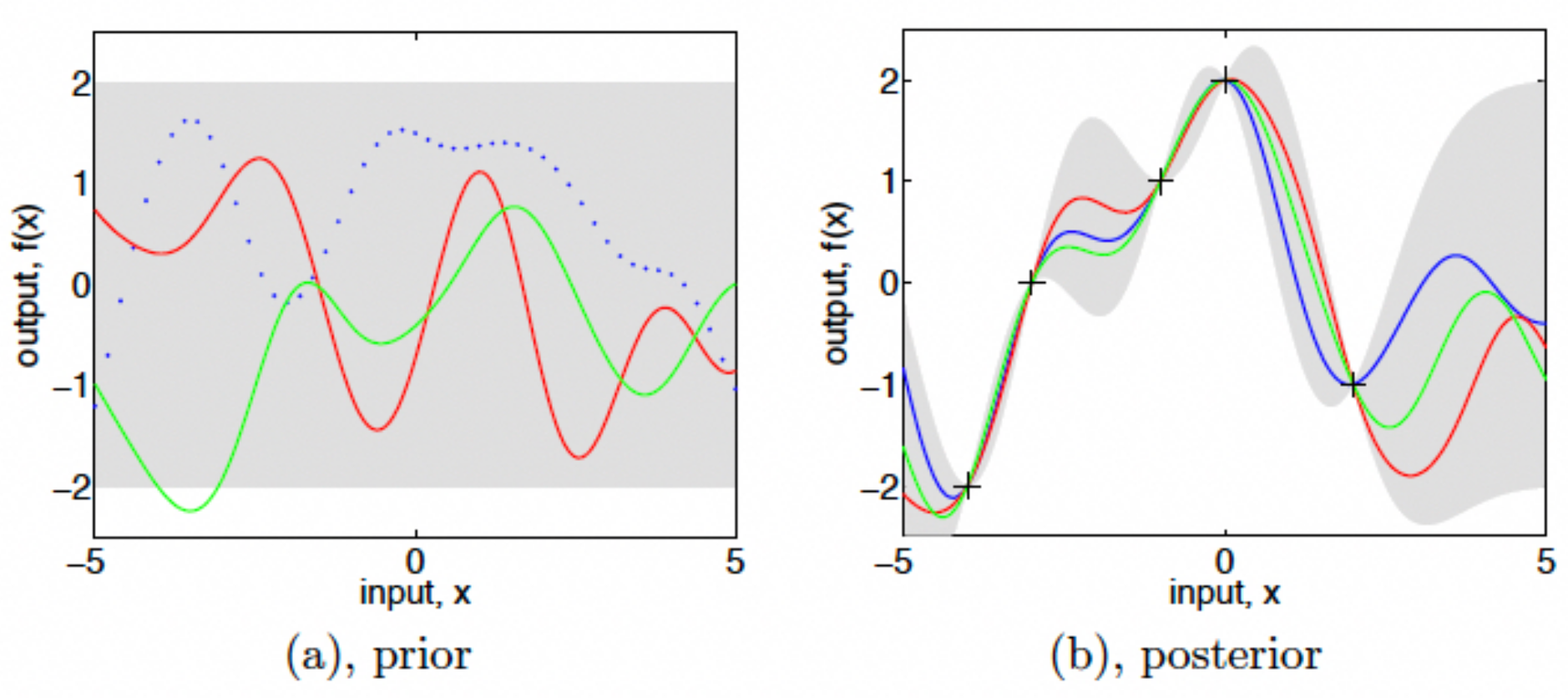
Figure: Gaussian process prior and posterior. “Panel (a) shows three functions drawn at random from a GP prior; the dots indicate values of y actually generated; the two other functions have (less correctly) been drawn as lines by joining a large number of evaluated points. Panel (b) shows three random functions drawn from the posterior, i.e. the prior conditioned on the five noise free observations indicated. In both plots the shaded area represents the pointwise mean plus and minus two times the standard deviation for each input value (corresponding to the 95% confidence region), for the prior and posterior respectively” (source: http://www.gaussianprocess.org/gpml/).#
Linear fitting#
Linear Regression#
A linear regression model just finds a linear relation between descriptors and the output. For more details see the book of mathematics of machine learning and book of Kevin Murphy or some other standard text books on machine learning.
More information of these implementations, specifically GPR will be added latter.